The Oracle JSON functions are very useful for generating JSON from a query, and developing using these functions requires understanding the limitations of the string data types they return.
Unless otherwise specified, they return a VARCHAR2 with a maximum of 4000 bytes. If your query might return more than this, you must either specify a larger length, e.g. RETURNING VARCHAR2(32767), or request a CLOB, e.g. RETURNING CLOB.
If the data exceeds the limit, calls to JSON_OBJECT, JSON_OBJECTAGG, JSON_ARRAYAGG, and JSON_TRANSFORM will fail at runtime with the following exception:
select
    json_object(
        'name-is-twenty-chars' : rpad('x',3974,'x')
    )
from dual;

ORA-40478: output value too large (maximum: 4000)
The error occurs here because the representation of the entire JSON object requires more than 4000 bytes. No-one likes to see errors, but it’s better than the alternative because it is more likely to alert you to the problem so you can fix it.
You may have noticed I missed one of the JSON functions from the list above – JSON_MERGEPATCH. By default, this function does not raise an exception if the size limit is exceeded. Instead, it merely returns NULL at runtime. This behaviour can cause confusion when debugging a complex query, so it’s something to be aware of.
Note that even though both the JSON objects specified RETURNING CLOB, this was missed for JSON_MERGEPATCH; which means it is limited to the default 4000 bytes, causing it to return NULL. The fix is to add RETURNING CLOB to the JSON_MERGEPATCH:
If you wish to remove a NOT NULL constraint from a column, normally you would execute this:
alter table t modify module null;
The other day a colleague trying to execute this on one of our tables encountered this error instead:
ORA-01451: column to be modified to NULL cannot be modified to NULL
*Cause:    the column may already allow NULL values, the NOT NULL constraint
           is part of a primary key or check constraint.
*Action:   if a primary key or check constraint is enforcing the NOT NULL
           constraint, then drop that constraint.
Most of the time when you see this error, it will be because of a primary key constraint on the column. This wasn’t the case for my colleague, however.
This particular column had a NOT NULL constraint. This constraint was not added deliberately by us; it had been applied automatically because the column has a default expression using the DEFAULT ON NULL option. For example:
create table t (
    ...
    module varchar2(64) default on null sys_context('userenv','module'),
    ...
);
A column defined with the DEFAULT ON NULL option means that if anything tries to insert a row where the column is null, or not included in the insert statement, the default expression will be used to set the column’s value. This is very convenient in cases where we always want the default value applied, even if some code tries to insert NULL into that column.
One would normally expect that a DEFAULT ON NULL implies that the column will never be NULL, so it makes sense that Oracle would automatically add a NOT NULL constraint on the column.
An edge case where this assumption does not hold true is when the default expression may itself evaluate to NULL; when that occurs, the insert will fail with ORA-01400: cannot insert NULL into ("SAMPLE"."T"."MODULE").
Therefore, my colleague wanted to remove the NOT NULL constraint, but their attempt failed with the ORA-01451 exception noted at the start of this article.
Unfortunately for us, the DEFAULT ON NULL option is not compatible with allowing NULLs for the column; so we had to remove the DEFAULT ON NULL option. If necessary, we could add a trigger on the table to set the column’s value if the inserted value is null.
The way to remove the DEFAULT ON NULL option is to simply re-apply the default, omitting the ON NULL option, e.g.:
alter table t modify module default sys_context('userenv','module');
Here’s a transcript illustrating the problem and its solution:
create table t (
    dummy number,
    module varchar2(64) default on null sys_context('userenv','module')
);

Table T created.

exec dbms_application_info.set_module('SQL Developer',null);

insert into t (dummy) values (1);

1 row inserted.

select * from t;

     DUMMY MODULE
---------- -----------------------------------------------------------
         1 SQL Developer


exec dbms_application_info.set_module(null,null);

insert into t (dummy) values (2);

Error report -
ORA-01400: cannot insert NULL into ("SAMPLE"."T"."MODULE")


alter table t modify module null;

ORA-01451: column to be modified to NULL cannot be modified to NULL


alter table t modify module default sys_context('userenv','module');

Table T altered.

insert into t (dummy) values (3);

1 row inserted.

select * from t;

     DUMMY MODULE
---------- -----------------------------------------------------------
         1 SQL Developer
         3
You are probably familiar with some of the data types supported by the Oracle Database for storing numeric values, but you might not be aware of the full range of types that it provides.
Some types (such as NUMBER, INTEGER) are provided for general use in SQL and PL/SQL, whereas others are only supported in PL/SQL (such as BINARY_INTEGER).
There are others (such as DECIMAL, REAL) that are provided to adhere to the SQL standard and for greater interoperability with other databases that expect these types.
Most of the numeric data types are designed for storing decimal numbers without loss of precision; whereas the binary data types (e.g. BINARY_FLOAT, BINARY_DOUBLE) are provided to conform to the IEEE754 standard for binary floating-point arithmetic. These binary types cannot store all decimal numbers exactly, but they do support some special values like “infinity” and “NaN”.
In PL/SQL you can define your own subtypes that further constrain the values that may be assigned to them, e.g. by specifying the minimum and maximum range of values, and/or by specifying that variables must be Not Null.
What do I prefer?
In my data models, I will usually use NUMBER to store numeric values, e.g. for quantities and measurements; for counts and IDs (e.g. for surrogate keys) I would use INTEGER (with the exception of IDs generated using sys_guid, these must use NUMBER).
In PL/SQL, if I need an index for an array, I will use BINARY_INTEGER (although if I’m maintaining a codebase that already uses its synonym PLS_INTEGER, I would use that for consistency). In other cases I will use INTEGER or NUMBER depending on whether I need to store integers or non-integers.
I don’t remember any occasion where I’ve needed to use FLOAT, or the binary types; and of the subtypes of BINARY_INTEGER, I’ve only used SIGNTYPE maybe once or twice. Of course, there’s nothing wrong with these types, it’s just that I haven’t encountered the need for them (yet).
What about Performance?
There are some differences in performance between these data types, but most of the time this difference will not be significant compared to other work your code is doing – see, for example, Connor on Choosing the Best Data Type. Choosing a data type that doesn’t use more storage than is required for your purpose can make a difference when the volume of data is large and when large sets of record are being processed and transmitted.
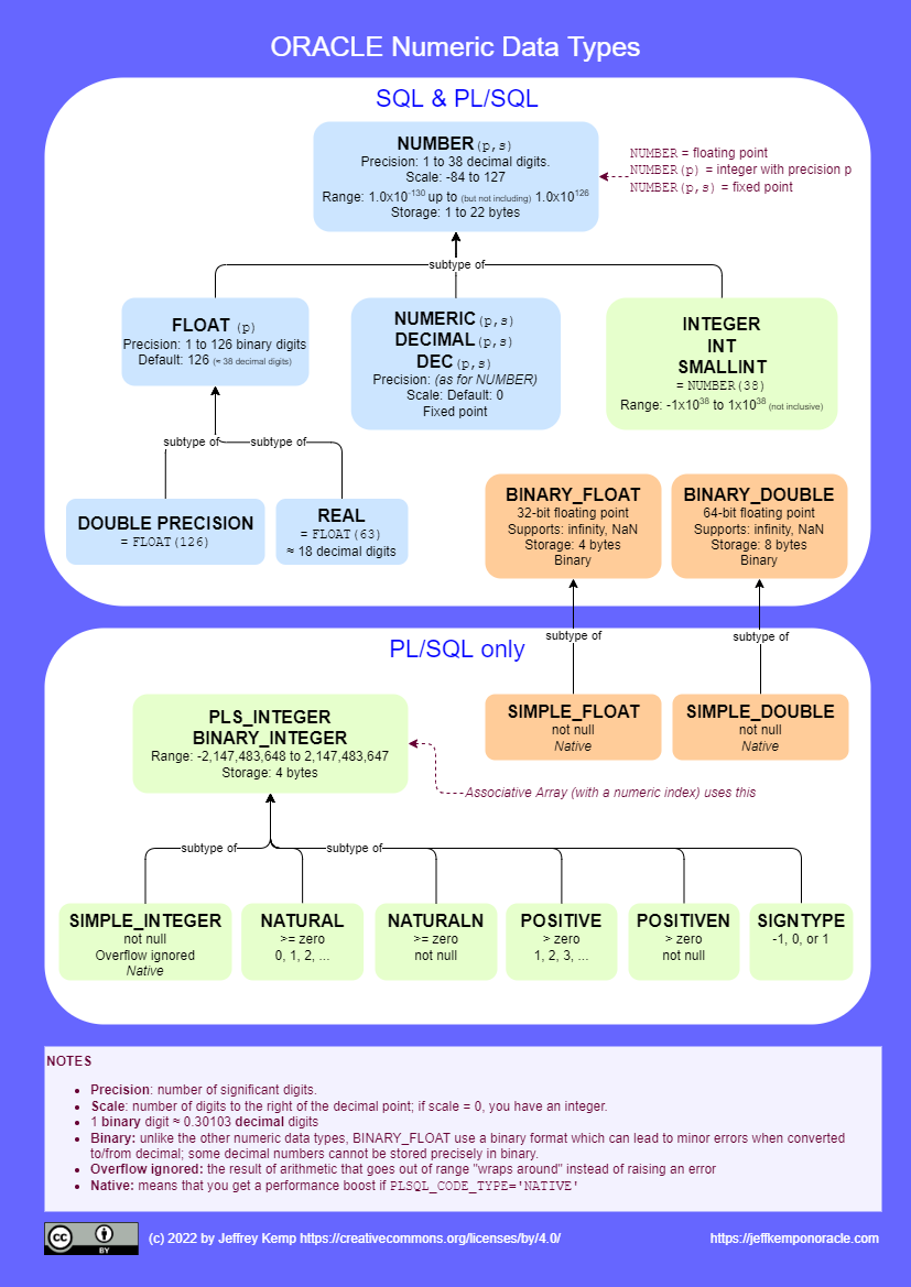
Reference Chart: Numeric Data Types
This diagram shows all the numeric data types supplied by Oracle SQL and PL/SQL, and how they relate to each other:
From smallest to largest – the maximum finite integer that can be stored by these data types is listed here. It’s interesting to see that BINARY_FLOAT can store bigger integers than INTEGER, but NUMBER can beat both of them:
BINARY_INTEGER
2.147483647 x 10⁹
INTEGER
9.9999999999999999999999999999999999999 x 1037
BINARY_FLOAT
3.40282347 x 1038
NUMBER
9.999999999999999999999999999999999999999 x 10125
BINARY_DOUBLE
1.7976931348623157 x 10308
To put that into perspective:
If you need to store integers up to about 1 Billion (109), you can use a BINARY_INTEGER.
If you need to store Googolplex (10googol) or other ridiculously large numbers (that are nevertheless infinitely smaller than infinity), you’re “gonna need a bigger boat” – such as some version of BigDecimal with a scale represented by a BigInteger – which unfortunately has no native support in SQL or PL/SQL. Mind you, there are numbers so large that even such an implementation of BigDecimal cannot even represent the number of digits in them…
Storing SMALL Numbers
The smallest non-zero numeric value (excluding subnormal numbers) that can be stored by these data types is listed here.
BINARY_FLOAT
1.17549435 x 10-38
NUMBER
1.0 x 10-130
BINARY_DOUBLE
2.2250738585072014 x 10-308
These are VERY small quantities. For example:
The size of a Quark, the smallest known particle, is less than 10-19 metres and can easily be represented by any of these types.
You can store numbers as small as the Planck Length (1.616 × 10⁻³⁵ metres) in a BINARY_FLOAT.
But to store a number like the Planck Time (5.4 × 10-44 seconds), you need a NUMBER – unless you change the units to nanoseconds, in which case it can also be stored in a BINARY_FLOAT.
I’m not aware of any specifically named numbers so small that they require a BINARY_DOUBLE; however, there are certainly use cases (e.g. scientific measurements) that need the kind of precision that this type provides.
If you break out into a sweat reading the title, it probably means that like me, you have had too little exposure to working with timestamps in Oracle.
Until recently I never really had much to do with time zones because I lived in the (now even moreso, due to covid) insular state of Western Australia. In WA most places pretend that there is no such thing as time zones – so our exposure to Oracle data types is limited to simple DATEs and TIMESTAMPs, with nary a time zone in sight. We just set the server time zone to AUSTRALIA/Perth and forget it.
Now I’ve helped build a system that needs to concurrently serve the needs of customers in any time zone – whether in the US, in Africa, or here in Australia. We therefore set the server time zone to UTC and use data types that support time zones, namely:
TIMESTAMP WITH TIME ZONE – for dates and times that need to include the relevant time zone; and
TIMESTAMP WITH LOCAL TIME ZONE – for dates and times of system events (e.g. record audit data) that we want to always be shown as of the session time zone (i.e. UTC), and we don’t care what time zone they were originally created in.
A colleague came to me with the following issue: a business rule needed to check an appointment date/time with the current date; if the appointment was for the prior day, an error message should be shown saying that they were too late for their appointment. A test case was failing and they couldn’t see why.
Here is the code (somewhat obfuscated):
if appointment_time < trunc(current_time) then
    :p1_msg := 'This appointment was for the previous day and has expired.';
end if;
We had used TRUNC here because we want to check if the appointment time was prior to midnight of the current date, from the perspective of the relevant time zone. The values of appointment_time and current_time seemed to indicate it shouldn’t fail:
appointment_time = 05-MAR-2021 07.00.00.000000 AM AUSTRALIA/Perth
current_time     = 05-MAR-2021 06.45.00.000000 AM AUSTRALIA/Perth
We can see that the appointment time and current time are in the same time zone, and the same day – so the tester expected no error message would be shown. (Note that the “current time” here is computed using localtimestamp at the time zone of the record being compared)
After checking that our assumptions were correct (yes, both appointment_time and current_time are TIMESTAMP WITH TIME ZONEs; and yes, they had the values shown above) we ran a query on the database to start testing our assumptions about the logic being run here.
select
    to_timestamp_tz('05-MAR-2021 07.00.00.000000 AM AUSTRALIA/Perth') as appt_time,
    to_timestamp_tz('05-MAR-2021 06.45.00.000000 AM AUSTRALIA/Perth') as current_time
from dual

APPT_TIME    = '05-MAR-2021 07.00.00.000000000 AM AUSTRALIA/PERTH'
CURRENT_TIME = '05-MAR-2021 06.45.00.000000000 AM AUSTRALIA/PERTH'
So far so good. What does an ordinary comparison show for these values?
with q as (
    select
        to_timestamp_tz('05-MAR-2021 07.00.00.000000 AM AUSTRALIA/Perth') as appt_time,
        to_timestamp_tz('05-MAR-2021 06.45.00.000000 AM AUSTRALIA/Perth') as current_time
    from dual)
select
    q.appt_time,
    q.current_time,
    case when q.appt_time < q.current_time then 'FAIL' else 'SUCCESS' end test
from q;

APPT_TIME    = '05-MAR-2021 07.00.00.000000000 AM AUSTRALIA/PERTH'
CURRENT_TIME = '05-MAR-2021 06.45.00.000000000 AM AUSTRALIA/PERTH'
TEST         = 'SUCCESS'
That’s what we expected; the appointment time is not before the current time, so the test is successful. Now, let’s test the expression actually used in our failing code, where the TRUNC has been added:
with q as (
    select
        to_timestamp_tz('05-MAR-2021 07.00.00.000000 AM AUSTRALIA/Perth') as appt_time,
        to_timestamp_tz('05-MAR-2021 06.45.00.000000 AM AUSTRALIA/Perth') as current_time
    from dual)
select
    q.appt_time,
    q.current_time,
    trunc(q.current_time),
    case when q.appt_time < trunc(q.current_time) then 'FAIL' else 'SUCCESS' end test
from q;

APPT_TIME           = '05-MAR-2021 07.00.00.000000000 AM AUSTRALIA/PERTH'
CURRENT_TIME        = '05-MAR-2021 06.45.00.000000000 AM AUSTRALIA/PERTH'
TRUNC(CURRENT_TIME) = '03/05/2021'
TEST                = 'FAIL'
Good: we have reproduced the problem. Now we can try to work out why it is failing. My initial suspicion was that an implicit conversion was causing the issue – perhaps the appointment date was being converted to a DATE prior to the comparison, and was somehow being converted to the UTC time zone, which was the database time zone?
with q as (
    select
        to_timestamp_tz('05-MAR-2021 07.00.00.000000 AM AUSTRALIA/Perth') as appt_time,
        to_timestamp_tz('05-MAR-2021 06.45.00.000000 AM AUSTRALIA/Perth') as current_time
    from dual)
select
    q.appt_time,
    q.current_time,
    cast(q.appt_time as date),
    cast(q.current_time as date)
from q;

APPT_TIME                  = '05-MAR-2021 07.00.00.000000000 AM AUSTRALIA/PERTH'
CURRENT_TIME               = '05-MAR-2021 06.45.00.000000000 AM AUSTRALIA/PERTH'
CAST(APPT_TIME AS DATE)    = '03/05/2021 07:00:00 AM'
CAST(CURRENT_TIME AS DATE) = '03/05/2021 06:45:00 AM'
Nope. When cast to a DATE, both timestamps still fall on the same date. Then I thought, maybe when a DATE is compared with a TIMESTAMP, Oracle first converts the DATE to a TIMESTAMP?
with q as (
    select
        to_timestamp_tz('05-MAR-2021 07.00.00.000000 AM AUSTRALIA/Perth') as appt_time,
        to_timestamp_tz('05-MAR-2021 06.45.00.000000 AM AUSTRALIA/Perth') as current_time
    from dual)
select
    q.appt_time,
    q.current_time,
    cast(trunc(q.current_time) as timestamp with time zone),
    case when q.appt_time < trunc(q.current_time) then 'FAIL' else 'SUCCESS' end test
from q;

APPT_TIME                              = '05-MAR-2021 07.00.00.000000000 AM AUSTRALIA/PERTH'
CURRENT_TIME                           = '05-MAR-2021 06.45.00.000000000 AM AUSTRALIA/PERTH'
CAST(TRUNC(CURRENT_TIME) AS TIMESTAMP) = '05-MAR-2021 12.00.00.000000 AM +00:00'
TEST                                   = 'FAIL'
Ah! Now we can see the cause of our problem. After TRUNCating a timestamp, we have converted it to a DATE (with no timezone information); since Oracle needs to implicitly convert this back to a TIMESTAMP WITH TIME ZONE, it simply slaps the UTC time zone on it. Now, when it is compared with the appointment time, it fails the test because the time is 12am (midnight) versus 7am.
Our original requirement was only to compare the dates involved, not the time of day; if the appointment was on the previous day (in the time zone relevant to the record), the error message should appear. We therefore need to ensure that Oracle performs no implicit conversion, by first converting the appointment time to a DATE:
with q as (
    select
        to_timestamp_tz('05-MAR-2021 07.00.00.000000 AM AUSTRALIA/Perth') as appt_time,
        to_timestamp_tz('05-MAR-2021 06.45.00.000000 AM AUSTRALIA/Perth') as current_time
    from dual)
select
    q.appt_time,
    q.current_time,
    case when cast(q.appt_time as date) < trunc(q.current_time) then 'FAIL' else 'SUCCESS' end test
from q;

APPT_TIME                              = '05-MAR-2021 07.00.00.000000000 AM AUSTRALIA/PERTH'
CURRENT_TIME                           = '05-MAR-2021 06.45.00.000000000 AM AUSTRALIA/PERTH'
TEST                                   = 'SUCCESS'
Our logic therefore should be:
if cast(appointment_time as date) < trunc(current_time) then
    :p1_msg := 'This appointment was for the previous day and has expired.';
end if;
It should be noted that if the tester had done this just an hour later in the day, they would not have noticed this problem – because Perth is +08:00, and the timestamps for the test data were prior to 8am in the morning.
Lesson #1: in any system that deals with timestamps and time zones it’s quite easy for subtle bugs to survive quite a bit of testing.
Lesson #2: when writing any comparison code involving timestamps and time zones, make sure that the data types are identical – and if they aren’t, add code to explicitly convert them first.
Need to run DBMS_MVIEW.explain_mview in APEX SQL Workshop, but don’t have the MV_CAPABILITIES_TABLE? You’ll get this error:
ORA-30377: table ORDS_PUBLIC_USER.MV_CAPABILITIES_TABLE not found
You don’t need to create this table. You could create this table by running admin/utlxmv.sql (if you have it). Instead, you can get the output in an array and do whatever you want with its contents, e.g.:
declare
    a sys.ExplainMVArrayType;
begin
    dbms_mview.explain_mview('MY_MV',a);
    dbms_output.put_line('Explain MV '
        || a(1).mvowner || '.' || a(1).mvname);
    for i in 1..a.count loop
        dbms_output.put_line(
            rpad(a(i).capability_name, 30)
            || ' [' || case a(i).possible
                       when 'T' then 'TRUE'
                       when 'F' then 'FALSE'
                       else a(i).possible
                       end || ']'
            || case when a(i).related_num != 0 then
                   ' ' || a(i).related_text
                   || ' (' || a(i).related_num || ')'
               end
            || case when a(i).msgno != 0 then
                   ' ' || a(i).msgtxt
                   || ' (' || a(i).msgno || ')'
               end
        );
    end loop;
end;
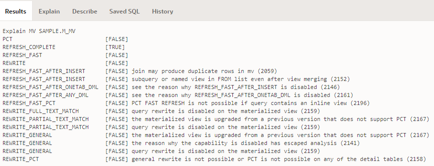
The result will be something like this:
Now, the challenge is merely how to resolve some of those “FALSEs” …
A good question – how to load fairly largish GeoJSON documents into a Google Map in APEX?
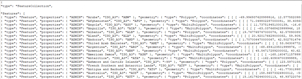
To investigate this I started by downloading a source of GeoJSON data for test purposes – one containing the borders of countries around the world: https://datahub.io/core/geo-countries. This file is 23.5MB in size and contains a JSON array of features, like this:
(the data does not appear to be very accurate for a lot of countries, but it will do just fine for my purposes)
Uploading the file to the database
To load this file into my database I copied the file to the server and ran this to load the data into a temporary table:
Alternatively, I could also have created a temporary APEX application with a File Browse item to upload the file and insert it into the import_lob_tmp table.
Parsing the JSON
I wanted to get the array of features as a table with one row per country; to get this I used json_table; after a fair bit of muddling around this is what I ended up with:
create table country_borders as
select j.*
from import_lob_tmp,
     json_table(the_clob, '$.features[*]'
         columns (
             country varchar2(255) path '$.properties.ADMIN',
             iso_a3 varchar2(255) path '$.properties.ISO_A3',
             geometry clob format json
         )) j;

alter table country_borders modify country not null;
alter table country_borders modify iso_a3 not null;
alter table country_borders modify geometry not null;
alter table country_borders add
    constraint country_border_name_uk unique (country);
alter table country_borders add
    constraint geometry_is_json check (geometry is json);
The first JSON path expression allowed me to drill down from the document root ($) to the features node; this is an array so I added [*] to get one row for each entry.
The COLUMNS list then breaks down each entry into the columns I’m interested in; each entry consists of a type attribute (which I don’t need), followed by a more interesting properties node with some attributes which are extracted using some relative JSON path expressions; followed by the geometry node with the GeoJSON fragment that represents the country borders that I wish to store “as is” in a clob column.
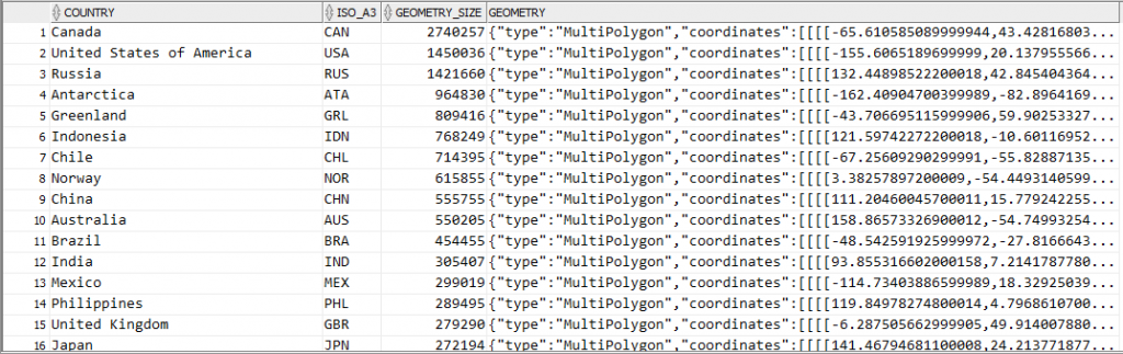
Now if I query this table it’s interesting to see which countries are likely to have the most complex coastlines (at least, as far as the data quality provided in this file will provide):
select country,
       iso_a3,
       dbms_lob.getlength(geometry) geometry_size,
       geometry
from country_borders
order by 3 desc;
It should be noted that since I’ve extracted the geometry node from each feature, the resulting data in the geometry column do not actually represent valid GeoJSON documents. However, it’s easy to construct a valid GeoJSON document by surrounding it with a suitable JSON wrapper, e.g.:
'{"type":"Feature","geometry":' + geometry + '}'
Showing the GeoJSON on a map
The next step is to load this border data onto a map for display. I recently released version 1.1 of my Report Map Google Map plugin which adds support for loading and manipulating geoJSON strings, so I started by importing region_type_plugin_com_jk64_report_google_map_r1 into my APEX application.
I created a page with a region using this plugin. I set the map region Static ID to testmap. On the same page I added a text item, P1_GEOJSON, to hold the GeoJSON data; and a Select List item P1_COUNTRY with the following query as its source:
select country
       || ' ('
       || ceil(dbms_lob.getlength(geometry)/1024)
       || 'KB)' as d
      ,country
from country_borders
order by country
I added a dynamic action to the Select List item on the Change event to load the geometry from the table into the map. Initially, I added the following actions:
A Set Value action that sets P1_GEOJSON to the result of the query: select geometry from country_borders where country = :P1_COUNTRY
An Execute JavaScript action that loads the GeoJSON into the map (after first clearing any previously loaded features):
This technique works ok, but only for smallish countries where the GeoJSON of their borders is less than 4K in size. For countries with more border detail than can fit within that limit, the Set Value action query only loads part of the JSON data, resulting in an invalid JSON string – and so the map failed to load it. The Set Value action was therefore unsuitable for my purpose.
To load the entire CLOB data I used another plugin. There are a few CLOB load plugins available for APEX – search the Plugins list at apex.world for “clob”. I chose APEX CLOB Load 2 by Ronny Weiß.
I imported the plugin dynamic_action_plugin_apex_clob_load_2 into my application, then replaced the Set Value action with the action APEX CLOB Load 2 [Plug-In]. I set SQL Source to:
select /* Element type dom - for jQuery selector e.g. body or #region-id,
          item - for item name e.g. P1_MY_ITEM */
       'item' as element_type,
       /* jQuery selector or item name */
       'P1_GEOJSON' as element_selector,
       geometry as clob_value
from country_borders
where country = :P1_COUNTRY
I set Items to Submit = P1_COUNTRY and Sanitise HTML = No. I also set Selection Type = Region and select the map region so that the spinner is shown while the data is loaded.
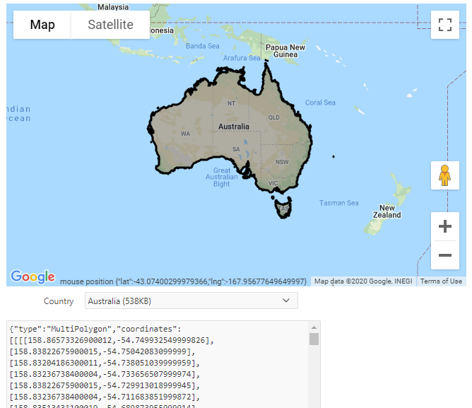
Result
The plugin works well. The border for any country can be loaded (for some countries, it takes a few extra seconds to load) and drawn on the map:
If you would like to see this in action, you may play with it here: https://jk64.dev/apex/f?p=JK64_REPORT_MAP:GEOJSON
Last year I *(not pictured) celebrated my 42nd circuit around the sun. In accordance with time-honoured tradition, it has been celebrated some time around the same day each September with variations on the following theme:
a get-together with friends and/or family
my favourite meal (usually lasagne)
my favourite cake (usually a sponge coffee torte, yum)
a gift or two
the taking of photographs, to document how much I’ve grown since the last one
Each year, determining the date this anniversary should fall on is a simple calculation combining the current year with the month and day-of-month. So, in the example of the special, but somewhat disadvantaged, people whose birthday falls on Christmas day (if you are among this select group, you have my sympathies), we could calculate their birthdays using a simple SQL expression like this:
with testdata as (
select date'2000-12-25' as d1
from dual)
select rownum-1 as age
      ,extract(day from d1)
       || '-' || to_char(d1,'MON')
       || '-' || (extract(year from d1)+rownum-1) as d1
from testdata connect by level <= 12;
Of course, as you should well know, this is wrong. It assumes that every year has every day that the anniversary might fall on. If a person is in that very special group of people who were born on the leap day of a leap year, our algorithm produces invalid dates in non-leap years:
with testdata as (
select date'2000-12-25' as d1
      ,date'2000-02-29' as d2
from dual)
select rownum-1 as age
      ,extract(day from d1)
       || '-' || to_char(d1,'MON')
       || '-' || (extract(year from d1)+rownum-1) as d1
      ,extract(day from d2)
       || '-' || to_char(d2,'MON')
       || '-' || (extract(year from d1)+rownum-1) as d2
from testdata connect by level <= 12;
This is because we are constructing a string which may or may not represent a real date in our crazy calendar system. So any self-respecting Oracle developer will know that the “correct” way of calculating this sort of thing is to use the ADD_MONTHS function, generously gifted to all of us for free:
with testdata as (
select date'2000-12-25' as d1
      ,date'2000-02-29' as d2
from dual)
select rownum-1 as age
      ,add_months(d1,12*(rownum-1)) as d1
      ,add_months(d2,12*(rownum-1)) as d2
from testdata connect by level <= 12;
Hurrah, we now have valid dates (this is guaranteed by ADD_MONTHS), and those poor souls born on a leap day can still celebrate their birthday, albeit on the 28th of the month in non-leap years. Some of the more pedantic of these might wait until the following day (the 1st of March) to celebrate their birthday, but for the purpose of our calculation here the 28th is a little simpler to work with.
We package up our software and deliver it to the customer, it passes all their tests and it goes into Production where it works quite fine – for about a week or so.
Someone notices that for SOME people, whose anniversary did NOT fall on a leap day but were born on the 28th of February, are being assigned the 29th of February as their day of celebration in every leap year. However, not everyone has this problem: other people whose birthday is also on the 28th of February are being correctly calculated as the 28th of February whether it’s a leap year or not.
Obviously there’s a bug in Oracle’s code, somewhere. Maybe. Well, not a bug so much, this is due to the way that ADD_MONTHS chooses to solve the problem of “adding one month” when a “month” is not defined with a constant number of days. ADD_MONTHS attempts to satisfy the requirements of most applications where if you start from the last day of one month, the result of ADD_MONTHS will also be the last day of its month. So add_months(date'2000-06-30', 1) = date'2000-07-31',add_months(date'2000-06-30', 1) = date'2000-07-30', and add_months(date'2000-05-31', 1) = date'2000-06-30'.
Let’s have a look at those dates. There’s one person whose birthday was 28 Feb 2000 and our algorithm is setting their anniversary as the 28th of February regardless of year. That’s fine. There’s another person who was born a year later on 28 Feb 2001, and our algorithm is setting their “gimme gimme” day to the 29th of February in each subsequent leap year. That’s not what we want.
with testdata as (
select date'2000-12-25' as d1
      ,date'2000-02-29' as d2
      ,date'2000-02-28' as d3
      ,date'2001-02-28' as d4
from dual)
select rownum-1 as age
      ,add_months(d1,12*(rownum-1)) as d1
      ,add_months(d2,12*(rownum-1)) as d2
      ,add_months(d3,12*(rownum-1)) as d3
      ,add_months(d4,12*(rownum-1)) as d4
from testdata connect by level <= 12;
Edge cases. Always with the edge cases. How shall we fix this? We’ll have to pick out those especially special people who were born on the 28th of February in a non-leap year and add some special handling.
with
  function birthday (d in date, age in number) return date is
  begin
    if to_char(d,'DD/MM') = '28/02'
    and to_char(add_months(d,age*12),'DD/MM') = '29/02'
    then
      return add_months(d,age*12)-1;
    else
      return add_months(d,age*12);
    end if;
  end;
select * from (
  with testdata as (
  select date'2000-12-25' as d1
        ,date'2000-02-29' as d2
        ,date'2000-02-28' as d3
        ,date'2001-02-28' as d4
  from dual)
  select rownum-1 as age
        ,birthday(d1,rownum-1) as d1
        ,birthday(d2,rownum-1) as d2
        ,birthday(d3,rownum-1) as d3
        ,birthday(d4,rownum-1) as d4
  from testdata connect by level <= 12
);
Now that’s what I call a happy birthday, for everyone – no matter how special.
p.s. that’s a picture of Tony Robbins at the top of this post. He’s a leap day kid. I don’t know when he celebrates his birthdays, but as he says, “the past does not equal the future.”
I received a question today from a developer who wanted to write a single static SQL query that could handle multiple optional parameters – i.e. the user might choose to leave one or more of the parameters NULL, and they’d expect the query to ignore those parameters. This is a quite common requirement for generic reporting screens, and there are two different methods commonly used to solve it.
Their sample query, using bind variables (natch), never returned any rows if any of the bind variables were null:
SELECT * FROM emp
WHERE job = :P_JOB
AND dept = :P_DEPT
AND city = :P_CITY
This is expected, of course, because “x = null” always evaluates to “unknown”, and this causes the rows to be omitted.
Option 1: add “OR v NOT NULL”, e.g.
SELECT * FROM emp
WHERE (job = :P_JOB OR :P_JOB IS NULL)
AND (dept = :P_DEPT OR :P_DEPT IS NULL)
AND (city = :P_CITY OR :P_CITY IS NULL)
Option 2: use NVL, e.g.
SELECT * FROM emp
WHERE job = NVL(:P_JOB, job)
AND dept = NVL(:P_DEPT, dept)
AND city = NVL(:P_CITY, city)
If the columns in the table do not have NOT NULL constraints on them, Option #2 will fail to return rows that have NULL in the relevant column – regardless of whether the user parameter is null or not. This is because “job = job” will always be “unknown” if job is null. In this case, Option #1 must be used.
If the columns do have NOT NULL constraints on them, then both Option #1 and Option #2 will work just fine. However, given the choice I would use Option #2 in order to take advantage of the potential performance optimisation that Oracle 12 can do with these types of NVL queries. There is a 3rd option, which is identical to Option #2 except that it uses the COALESCE function instead of NVL – but I would avoid this option as it will not get the performance optimisation.
On the other hand, if any of the attributes is the result of a costly operation (e.g. a function call), I would always use Option #1 (“OR NULL”) instead, because the NVL does not use short-circuit evaluation to avoid multiple function calls.
If there is a mix of columns that have NOT NULL constraints and others that don’t, I don’t really see any problem with mixing the two methods, e.g. in the case where dept has a NOT NULL constraint but job and city don’t:
SELECT * FROM emp
WHERE (job = :P_JOB OR :P_JOB IS NULL)
AND dept = NVL(:P_DEPT, dept)
AND (city = :P_CITY OR :P_CITY IS NULL)
Here’s a question for you to think about. What if the business rule states that the report should omit records where a column is null (i.e. the column may have nulls but they don’t want those records to ever appear in the report)? You may as well use NVL, e.g. in the case where dept has a NOT NULL constraint, but job and city don’t, but the report should omit records where job is null:
SELECT * FROM emp
WHERE job = NVL(:P_JOB, job)
AND dept = NVL(:P_DEPT, dept)
AND (city = :P_CITY OR :P_CITY IS NULL)
You might argue that future developers might be confused by the above query; it’s not exactly clear whether the developer intended to omit the records with null jobs, or if they made a mistake. Code comments might help, but alternatively you might choose to make the rule explicit, e.g.:
SELECT * FROM emp
WHERE job = NVL(:P_JOB, job) AND job IS NOT NULL
AND dept = NVL(:P_DEPT, dept)
AND (city = :P_CITY OR :P_CITY IS NULL)
If you feel strongly about this one way or another, please leave your comments below 🙂
This topic is a reminder that when there are multiple possible solutions to a problem, the choice should not be taken arbitrarily; and we should avoid enshrining one choice in any standards document as the “one true way”. This is because the answer is often “it depends” – different options may be valid for different scenarios, and have advantages and disadvantages that need to be taken into account.
The order in which your deployment scripts create views is important. This is a fact that I was reminded of when I had to fix a minor issue in the deployment of version #2 of my application recently.
Normally, you can just generate a create or replace force view script for all your views and just run it in each environment, then recompile your schema after they’re finished – and everything’s fine. However, if views depend on other views, you can run into a logical problem if you don’t create them in the order of dependency.
Software Release 1.0
create table t (id number, name varchar2(100));
create or replace force view tv_base as
select t.*, 'hello' as stat from t;
create or replace force view tv_alpha as
select t.* from tv_base t;

desc tv_alpha;
Name Null Type
---- ---- -------------
ID        NUMBER
NAME      VARCHAR2(100)
STAT      CHAR(5)
Here we have our first version of the schema, with a table and two views based on it. Let’s say that the tv_base includes some derived expressions, and tv_alpha is intended to do some joins on other tables for more detailed reporting.
Software Release 1.1
alter table t add (phone varchar2(10));
create or replace force view tv_alpha as
select t.* from tv_base t;
create or replace force view tv_base as
select t.*, 'hello' as stat from t;
Now, in the second release of the software, we added a new column to the table, and duly recompiled the views. In the development environment the view recompilation may happen multiple times (because other changes are being made to the views as well) – and nothing’s wrong. Everything works as expected.
However, when we run the deployment scripts in the Test environment, the “run all views” script has been run just once; and due to the way it was generated, the views are created in alphabetical order – so tv_alpha was recreated first, followed by tv_base. Now, when we describe the view, we see that it’s missing the new column:
desc tv_alpha;
Name Null Type
---- ---- -------------
ID        NUMBER
NAME      VARCHAR2(100)
STAT      CHAR(5)
Whoops. What’s happened, of course, is that when tv_alpha was recompiled, tv_base still hadn’t been recompiled and so it didn’t have the new column in it yet. Oracle internally defines views with SELECT * expanded to list all the columns. The view won’t gain the new column until we REPLACE the view with a new one using SELECT *. By that time, it’s too late for tv_alpha – it had already been compiled, successfully, so it doesn’t see the new column.
Lesson Learnt
What should we learn from this? Be wary of SELECT * in your views. Don’t get me wrong: they are very handy, especially during initial development of your application; but they can surprise you if not handled carefully and I would suggest it’s good practice to expand those SELECT *‘s into a discrete list of columns.
Some people would go so far as to completely outlaw SELECT *, and even views-on-views, for reasons such as the above. I’m not so dogmatic, because in my view there are some good reasons to use them in some situations.
I’ve been aware of some of the ways that Oracle database optimises index accesses for queries, but I’m also aware that you have to test each critical query to ensure that the expected optimisations are taking effect.
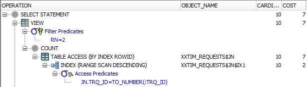
I had this simple query, the requirement of which is to get the “previous status” for a record from a journal table. Since the journal table records all inserts, updates and deletes, and this query is called immediately after an update, to get the previous status we need to query the journal for the record most recently prior to the most recent record. Since the “version_id” column is incremented for each update, we can use that as the sort order.
select status_code
from (select rownum rn, status_code
      from   xxtim_requests$jn jn
      where  jn.trq_id = :trq_id
      order by version_id desc)
where rn = 2;
The xxtim_requests$jn table has an ordinary index on (trq_id, version_id). This query is embedded in some PL/SQL with an INTO clause – so it will only fetch one record (plus a 2nd fetch to detect TOO_MANY_ROWS which we know won’t happen).
The table is relatively small (in dev it only has 6K records, and production data volumes are expected to grow very slowly) but regardless, I was pleased to find that (at least, in Oracle 12.1) it uses a nice optimisation so that it not only uses the index, it is choosing to use a Descending scan on it – which means it avoids a SORT operation, and should very quickly return the 2nd record that we desire.
It looks quite similar in effect to the “COUNT STOPKEY” optimisation you can see on “ROWNUM=1” queries. If this was a much larger table and this query needed to be faster or was being run more frequently, I’d probably consider appending status_code to the index in order to avoid the table access. In this case, however, I don’t think it’s necessary.


 The order in which your deployment scripts create views is important. This is a fact that I was reminded of when I had to fix a minor issue in the deployment of version #2 of my application recently.